MATLAB - Polynomials

MATLAB represents polynomials as row vectors containing coefficients ordered by descending powers. For example, the equation P(x) = x⁴ + 7x³ - 5x + 9 could be represented as:
p = [1 7 0 -5 9];

Evaluating Polynomials

The polyval function is used for evaluating a polynomial at a specified value. For example, to evaluate our previous polynomial p, at x = 4, type:

p = [1 7 0  -5 9];
polyval(p,4)

MATLAB executes the above statements and returns the following result:

ans =
   693

MATLAB also provides the polyvalm function for evaluating a matrix polynomial. A matrix polynomial is a polynomial with matrices as variables.
For example, let us create a square matrix X and evaluate the polynomial p, at X:

p = [1 7 0  -5 9];
X = [1 2 -3 4; 2 -5 6 3; 3 1 0 2; 5 -7 3 8];
polyvalm(p, X)

MATLAB executes the above statements and returns the following result:

ans =
        2307       -1769        -939        4499
        2314       -2376        -249        4695
        2256       -1892        -549        4310
        4570       -4532       -1062        9269

Finding the Roots of Polynomials

The roots function calculates the roots of a polynomial. For example, to calculate the roots of our polynomial p, type:

p = [1 7 0  -5 9];
r = roots(p)

MATLAB executes the above statements and returns the following result:

r =
  -6.8661 + 0.0000i
  -1.4247 + 0.0000i
   0.6454 + 0.7095i
   0.6454 - 0.7095i

The function poly is an inverse of the roots function and returns to the polynomial coefficients. For example:

p2 = poly(r)

MATLAB executes the above statements and returns the following result:

p2 =
    1.0000    7.0000    0.0000   -5.0000    9.0000

Polynomial Curve Fitting

The polyfit function finds the coefficients of a polynomial that fits a set of data in a least-squares sense. If x and y are two vectors containing the x and y data to be fitted to a n-degree polynomial, then we get the polynomial fitting the data by writing:

p = polyfit(x,y,n)

Example

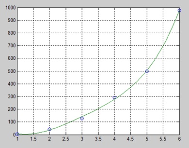
Create a script file and type the following code:

x = [1 2 3 4 5 6]; y = [5.5 43.1 128 290.7 498.4 978.67];  %data
p = polyfit(x,y,4)   %get the polynomial
% Compute the values of the polyfit estimate over a finer range, 
% and plot the estimate over the real data values for comparison:
x2 = 1:.1:6;          
y2 = polyval(p,x2);
plot(x,y,'o',x2,y2)
grid on

When you run the file, MATLAB displays the following result:

p =
    4.1056  -47.9607  222.2598 -362.7453  191.1250

And plots the following graph: