Simulink is a simulation and model-based design environment for
dynamic and embedded systems, integrated with MATLAB. Simulink, also
developed by MathWorks, is a data flow graphical programming language
tool for modeling, simulating and analyzing multi-domain dynamic
systems. It is basically a graphical block diagramming tool with
customizable set of block libraries.
It allows you to incorporate MATLAB algorithms into models as well as export the simulation results into MATLAB for further analysis.
Simulink supports:
The following list gives brief description of some of them:
Simulink Design Verifier allows you identify design errors and generates test case scenarios for model checking.
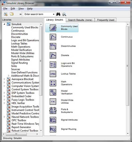 On the left side window pane, you will find several libraries
categorized on the basis of various systems, clicking on each one will
display the design blocks on the right window pane.
On the left side window pane, you will find several libraries
categorized on the basis of various systems, clicking on each one will
display the design blocks on the right window pane.
 A Simulink model is a block diagram.
Model elements are added by selecting the appropriate elements from the Library Browser and dragging them into the Model window.
Alternately, you can copy the model elements and paste them into the model window.
For the purpose of this example, 2 blocks will be used for the simulation - A Source (a signal) and a Sink (a scope). A signal generator (the source) generates an analog signal, which will then be graphically visualized by the scope(the sink).
 Begin by dragging the required blocks from the library to the project
window. Then, connect the blocks together which can be done by dragging
connectors from connection points on one block to those of another.
Begin by dragging the required blocks from the library to the project
window. Then, connect the blocks together which can be done by dragging
connectors from connection points on one block to those of another.
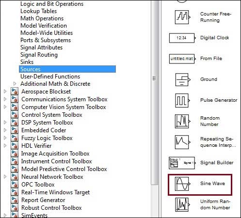
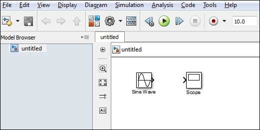
Let us drag a 'Sine Wave' block into the model.
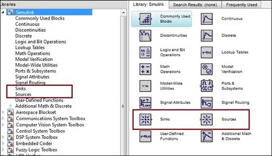
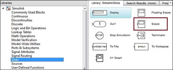
 Select 'Sinks' from the library and drag a 'Scope' block into the model.
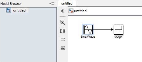
 Drag a signal line from the output of the Sine Wave block to the input of the Scope block.
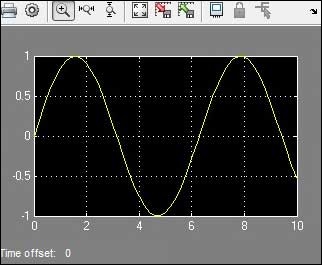
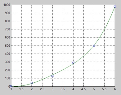
 Run the simulation by pressing the 'Run' button, keeping all parameters default (you can change them from the Simulation menu)
You should get the below graph from the scope.
It allows you to incorporate MATLAB algorithms into models as well as export the simulation results into MATLAB for further analysis.
Simulink supports:
- system-level design
- simulation
- automatic code generation
- testing and verification of embedded systems
The following list gives brief description of some of them:
- Stateflow allows developing state machines and flow charts.
- Simulink Coder allows to automatically generate C source code for real-time implementation of systems.
- xPC Target together with x86-based real-time systems provides an environment to simulate and test Simulink and Stateflow models in real-time on the physical system.
- Embedded Coder supports specific embedded targets.
- HDL Coder allows to automatically generate synthesizable VHDL and Verilog
- SimEvents provides a library of graphical building blocks for modeling queuing systems
Simulink Design Verifier allows you identify design errors and generates test case scenarios for model checking.
Using Simulink
To open Simulink, type in the MATLAB work space:simulink
Simulink opens with the Library Browser. The Library Browser is used for building simulation models.
On the left side window pane, you will find several libraries
categorized on the basis of various systems, clicking on each one will
display the design blocks on the right window pane. Building Models
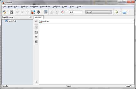
To create a new model, click the New button on the Library Browser's toolbar. This opens a new untitled model window
A Simulink model is a block diagram.Model elements are added by selecting the appropriate elements from the Library Browser and dragging them into the Model window.
Alternately, you can copy the model elements and paste them into the model window.
Examples
Drag and drop items from the Simulink library to make your project.For the purpose of this example, 2 blocks will be used for the simulation - A Source (a signal) and a Sink (a scope). A signal generator (the source) generates an analog signal, which will then be graphically visualized by the scope(the sink).
Begin by dragging the required blocks from the library to the project
window. Then, connect the blocks together which can be done by dragging
connectors from connection points on one block to those of another.Let us drag a 'Sine Wave' block into the model.
Select 'Sinks' from the library and drag a 'Scope' block into the model.
Drag a signal line from the output of the Sine Wave block to the input of the Scope block.
Run the simulation by pressing the 'Run' button, keeping all parameters default (you can change them from the Simulation menu)You should get the below graph from the scope.
 and displays the following result:
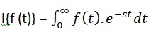 Laplace transform is also denoted as transform of f(t) to F(s). You
can see this transform or integration process converts f(t), a function
of the symbolic variable t, into another function F(s), with another
variable s.
Laplace transform is also denoted as transform of f(t) to F(s). You
can see this transform or integration process converts f(t), a function
of the symbolic variable t, into another function F(s), with another
variable s.  And displays the following result:
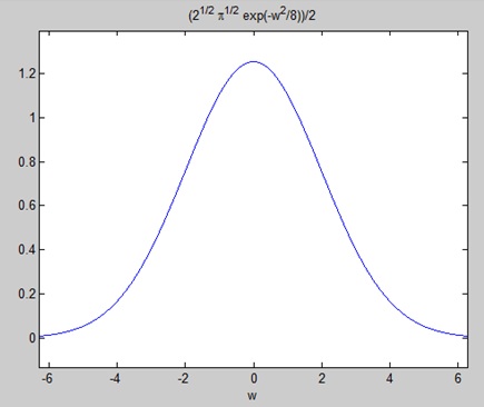
 we write,
 we write:
 Create a script file and type the following code:
 Here is Octave equivalent code for the above example:
 Here is Octave equivalent code for the above example:
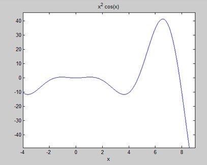
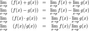 Let us consider two functions:
 and displays the following output: